A Beginner’s Guide to Quantum Computing and Python | Towards data science

Quantum Mechanics is the basic study of physics that describes phenomena on a microscopic scale (such as atoms and subatomic particles). This “new” field (1900) differs from Classical Physics, which describes nature on a large scale (such as bodies and machines) and does not work at the quantum level.

Quantum Computing it is a misuse of the properties of Quantum Mechanics to perform calculations and solve problems that an old computer cannot and will never do.

Conventional computers speak a binary code language: they assign a pattern of binary numbers (1s and 0s) to each character and instruction, and store and process that information in pieces. Even your Python code is converted to binary numbers when it runs on your laptop. For example:

The word “Hi” → “h”: 01001000 and “is”: 01101001 → 01001000 01101001

On the other hand, quantum computers process information by qubits (quantum bits), which can be 0 and 1 at the same time. That makes quantum machines much faster than conventional ones for certain problems (ie probabilistic computation).

Quantum computers

Quantum computers use atoms and electrons, instead of traditional silicon chips. As a result, they can use Quantum Mechanics to perform calculations faster than conventional machines. For example, 8 bits are enough for a classical computer to represent any number between 0 and 255, but 8-qubits are enough for a quantum computer to represent every number between 0 and 255. at the same time. A few hundred qubits would be enough to represent more numbers than there are atoms in the universe.

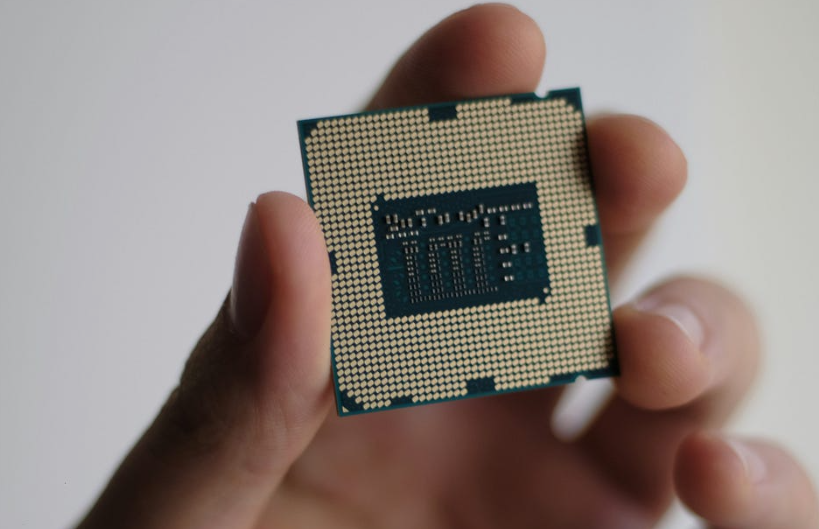
The brain of a quantum computer is tiny qubit chip made of steel or sapphire.

However, the most unique part is the large gold-plated cooling devices that look like a lamp hanging inside a metal cylinder: dilution refrigerator. It cools the chip to a temperature colder than the outside when the temperature destroys the quantum state (actually the colder, the more accurate).

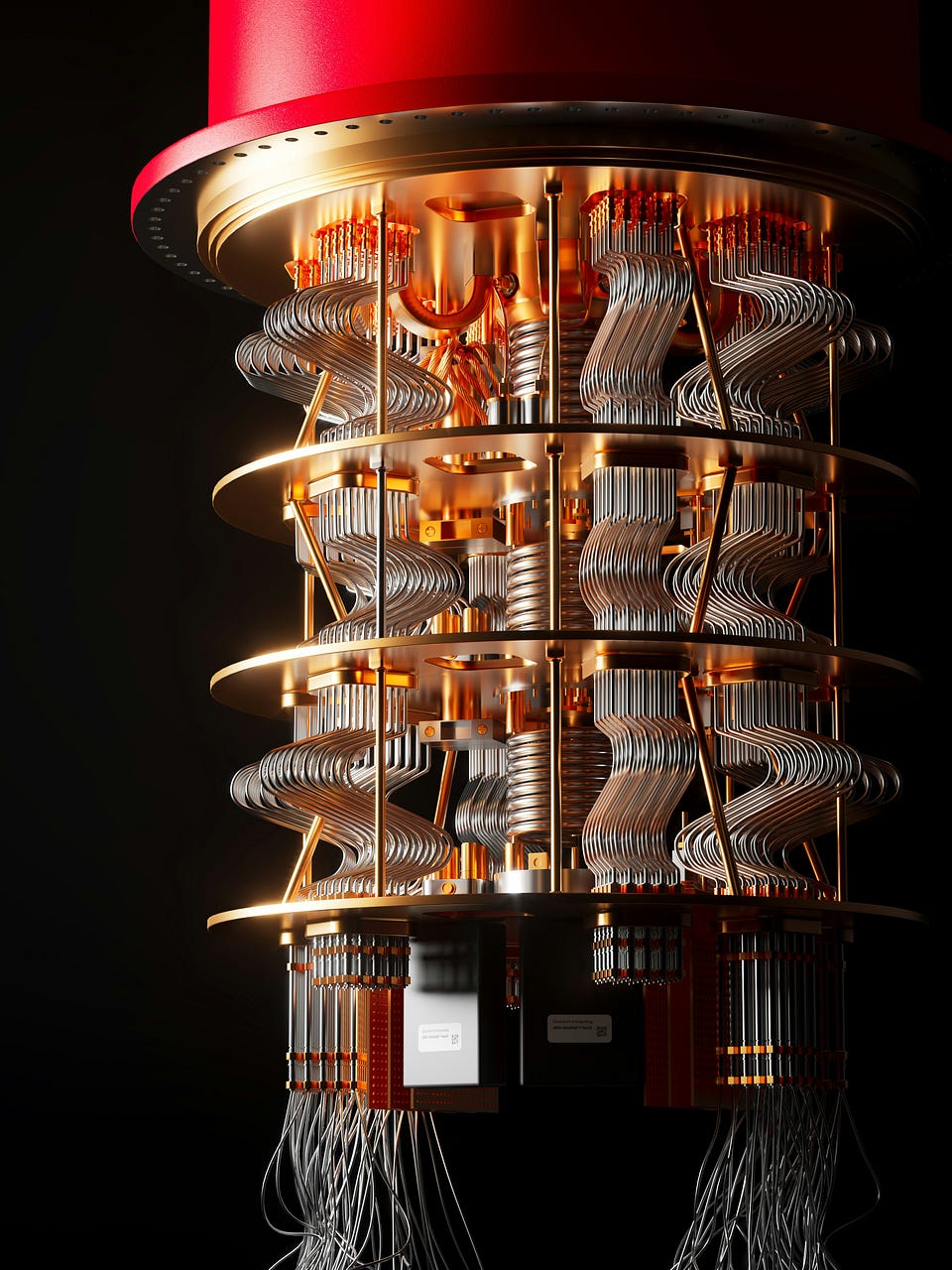
This is the main type of architecture, and it is called superconducting-qubits: artificial atoms made from circuits using superconductors (such as aluminum) that show zero electrical resistance at very low temperatures. Another design method is ion-traps (charged atoms trapped in electric fields in a very high vacuum), which are more accurate but slower than the first.

There is no accurate public count of how many quantum computers there are, but estimates are around 200 worldwide. As of today, the most advanced are:

1. Image of IBM Condorthe largest number of qubits built so far (1000 qubits), although that alone does not amount to significant figures as the error rates are still significant.
2. of Google Willoww (105 qubits), which has a good error rate but is still far from a fault-tolerant supercomputer.
3. ionQ of Tempo (100 qubits), an ion-traps quantum computer with great efficiency but still much slower than superconducting machines.
4. The quantinum’s Helios (98 qubits), using ion-trap designs with some of the highest precision reported today.
5. Picture of Rigetti Computing sample (80 kg).
6. of Intel Tunnel Falls (12 kilograms).
7. Canada Xanadu’s Aurora (12 qubits), the first photonic quantum computer, which uses light instead of electrons to process information.
8. Microsoft’s Majoranathe first computer designed for up to a million qubits on a single chip (but only 8 qubits currently).
9. Chinese SpinQs Minithe first portable small-scale quantum computer (2 qubits).
10. NVIDIA CPU (Center for Quantum Processing), the first quantum-fast GPU system.

Currently, it is not possible for the average person to own a large quantum computer, but you can get one in the cloud.

Arrangement

In Python, there are several libraries for working with quantum computers around the world:

• Kiskit by IBM is the most complete state-of-the-art ecosystem for running quantum programs on IBM quantum computers, ideal for beginners.
• Cirq by Google, dedicated to low-level control of their hardware, suitable for research.
• Penny Lane is Xanadu working hard on Quantum Machine Learning, it works on their photo computers but can connect with other providers.
• ProjectQ by ETH Zurich University, an open-source project that aims to be a basic package for general-purpose quantum computing.

For this tutorial, I will be using IBM’s Kiskit as an industry leader (pip install qiskit).

The most basic code we can write is to create a how much it rotates (an environment for quantum computation) with only one qubit and initialize it to 0. In order to measure the state of a qubit, we need statevectorwhich basically tells you the current quantum reality of your circuit.

from qiskit import QuantumCircuit
from qiskit.quantum_info import Statevector

q = QuantumCircuit(1,0) #circuit with 1 quantum bit and 0 classic bit
state = Statevector.from_instruction(q) #measure state
state.probabilities() #print prob%

It means: the probability that the qubit is 0 (the first object) is 100%, while the probability that the qubit is 1 (the second object) is 0%. You can print it like this:

print(f"[q=0 {round(state.probabilities()[0]*100)}%, 
         q=1 {round(state.probabilities()[1]*100)}%]")

Let’s visualize the situation:

from qiskit.visualization import plot_bloch_multivector

plot_bloch_multivector(state, figsize=(3,3))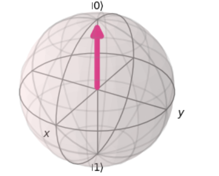

As you can see in the 3D picture of the quantum state, the qubit is 100% to 0. That was the equivalent of “Hello World“, and now we can move on to the quantum equivalent of “1+1=2“.

Qubits

Qubits have two fundamental properties of Quantum Mechanics: Superposition and Entanglement.

High level – old bits can be 1 or 0, but never both. On the contrary, a qubit can be both (technically it is an equal combination of an infinite number of states between 1 and 0), and as long as they are measured, the superposition falls to 1 or 0 and remains so forever. This is because the act of observing a quantum particle forces it to take on a binary state of 1 or 0 (especially the story of Schrödinger’s cat that we all know and love). Therefore, a qubit has a certain probability of falling to either 1 or 0.

q = QuantumCircuit(1,0)
q.h(0) #add Superposition
state = Statevector.from_instruction(q) 
print(f"[q=0 {round(state.probabilities()[0]*100)}%, 
         q=1 {round(state.probabilities()[1]*100)}%]")
plot_bloch_multivector(state, figsize=(3,3))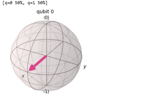

In the superposition, we introduced “randomness”, so the level of the vector is between 0 and 1. Instead of a vector image, we can use a q-sphere where the size of the points is equal to the probability of the term corresponding to the state.

from qiskit.visualization import plot_state_qsphere

plot_state_qsphere(state, figsize=(4,4))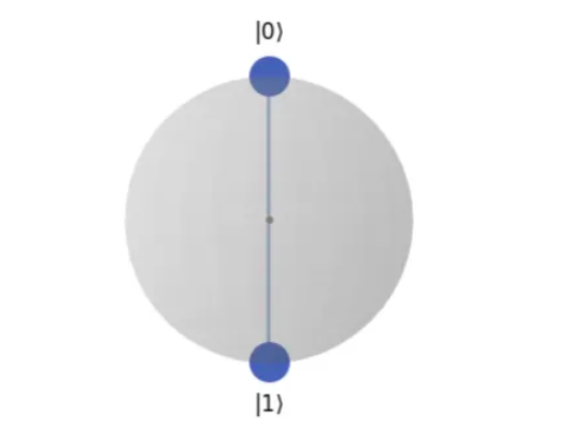

The qubit is both 0 and 1, with 50% probability respectively. But what happens if we measure it? Sometimes it will be a fixed 1, and sometimes it will be a fixed 0.

result, collapsed = state.measure() #Superposition disappears
print("measured:", result)
plot_state_qsphere(collapsed, figsize=(4,4)) #plot collapsed state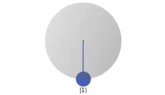

Entering – primitive bits are independent of each other, while qubits can be manipulated. When that happens, the qubits are forever connected, no matter how far apart they are (often used as a mathematical metaphor for love).

q = QuantumCircuit(2,0) #circuit with 2 quantum bits and 0 classic bit
q.h([0]) #add Superposition on the 1st qubit
state = Statevector.from_circuit(q) 
plot_bloch_multivector(state, figsize=(3,3))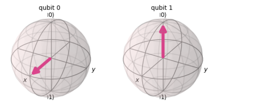

We have the first qubit in Superposition between 0-1, the second at 0, and now I’m going to add them. Therefore, if the first part is measured and falls to 1 or 0, the second part will change again (not necessarily the same result, one can be 0 and the other 1).

q.cx(control_qubit=0, target_qubit=1) #Entanglement
state = Statevector.from_circuit(q)
result, collapsed = state.measure([0]) #measure the 1st qubit
plot_bloch_multivector(collapsed, figsize=(3,3))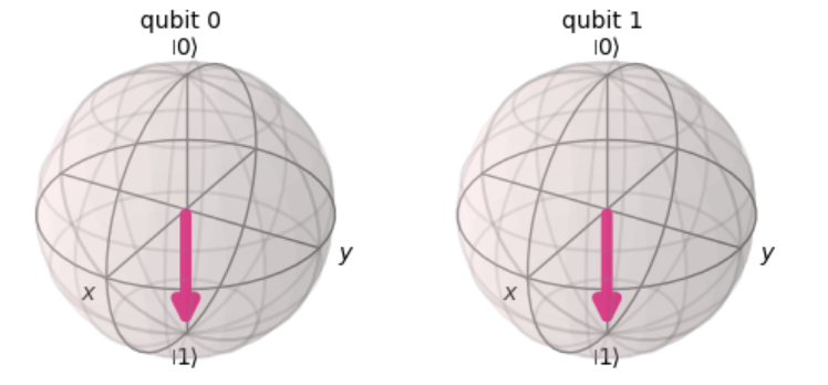

As you can see, the first qubit that was in Superposition was measured and fell to 1. At the same time, the second qubit is Entangled with the first, so it has changed again.

The end

This article has been a lesson in introduce the basics of Quantum Computing with Python and Qiskit. We learned how to work with qubits and their 2 main properties: Superposition and Entanglement. In the next lesson, we will use qubits to build quantum models.

Full code for this article: GitHub

I hope you enjoyed it! Feel free to contact me for questions and comments or to share your interesting projects.

👉 Let’s Connect 👈

_{^{(All images are by the author unless otherwise noted)}}